Reaction-diffusion systems explain how simple local rules can create large-scale biological and organic-looking structure. Two or more substances spread through space, react with each other, and repeatedly change the conditions for the next moment. Nothing in the equations explicitly says “make a stripe” or “grow a coral branch.” The pattern appears because diffusion smooths concentrations while reaction terms amplify some local differences and erase others.

This is one reason reaction-diffusion models are useful across mathematics, biology, chemistry, and generative art. They give a concrete way to study how local interactions can organize a surface without a central designer. The same idea is often used to discuss animal coat patterns, seashell pigmentation, chemical oscillations, tissue growth, and procedural texture generation. The exact biological systems are more complicated than the small simulation here, but the core intuition transfers well: a pattern can be a dynamic equilibrium between spreading and local transformation.

This article uses the Gray-Scott model, a common two-chemical reaction-diffusion system. It is compact enough to simulate interactively, but rich enough to produce spots, stripes, labyrinths, fronts, and unstable chaotic regions. You will paint initial chemical distributions, adjust parameters live, control time evolution, and compare stable and unstable regions side by side.

Two Chemicals, Local Reactions, and Diffusion

The model tracks two concentration fields, usually called $A$ and $B$. Think of them as two chemicals distributed over a thin surface. At every grid cell, the values change because of two processes:

1. Diffusion moves each chemical from high concentration toward low concentration.
2. Reaction converts chemicals based on the local amounts of $A$ and $B$.

The Gray-Scott equations are commonly written as:

$$\frac{\partial A}{\partial t} = D_A\nabla^2 A - AB^2 + f(1 - A)$$ $$\frac{\partial B}{\partial t} = D_B\nabla^2 B + AB^2 - (k + f)B$$

The notation looks dense, but each term has a direct job. $D_A\nabla^2 A$ and $D_B\nabla^2 B$ are diffusion terms. They spread each chemical according to nearby concentrations. The $AB^2$ term is the local reaction: chemical $B$ grows when it has enough of itself and chemical $A$ nearby, while $A$ is consumed. The parameter $f$ feeds fresh $A$ into the system. The parameter $k$ removes $B$ from the system.

That feed-and-removal balance is what makes the model interesting. If $B$ disappears too quickly, the field returns to a mostly uniform state. If $B$ persists and reproduces too aggressively, fronts can spread, split, and interfere. Between those extremes, the system can settle into regular spots, stripes, rings, or branching structures.

Painting the Initial Distribution

The first important lesson is that the initial state matters, but it does not control every detail. When you paint chemical $B$ into a field mostly filled with $A$, the painted region does not simply stay where you put it. The boundary becomes active. $B$ consumes nearby $A$, diffusion spreads both chemicals, and the reaction term reinforces some edge regions while starving others.

Drag across the canvas to inject chemical $B$. Small strokes tend to become islands, rings, or short bands. Larger connected strokes often break into textured fronts because the interior and boundary experience different concentrations. The Brush radius control changes how wide the initial disturbance is. The Feed control changes how quickly fresh $A$ returns to the field, so it strongly affects whether painted areas fade, stabilize, or keep producing structure.

This is a useful way to think about many pattern-formation problems. An organism, chemical surface, or synthetic material may not need a detailed global blueprint. It may need local substances, local reaction rules, and a growth environment that keeps the system away from a completely uniform state. The initial disturbance starts the process, but the ongoing local dynamics shape the final pattern.

Feed and Kill Parameters as Pattern Controls

In the Gray-Scott model, feed and kill are the most visible controls. Feed replenishes chemical $A$. Kill removes chemical $B$. Together they define whether $B$ can maintain itself, whether it expands as a front, and whether it settles into repeated structures.

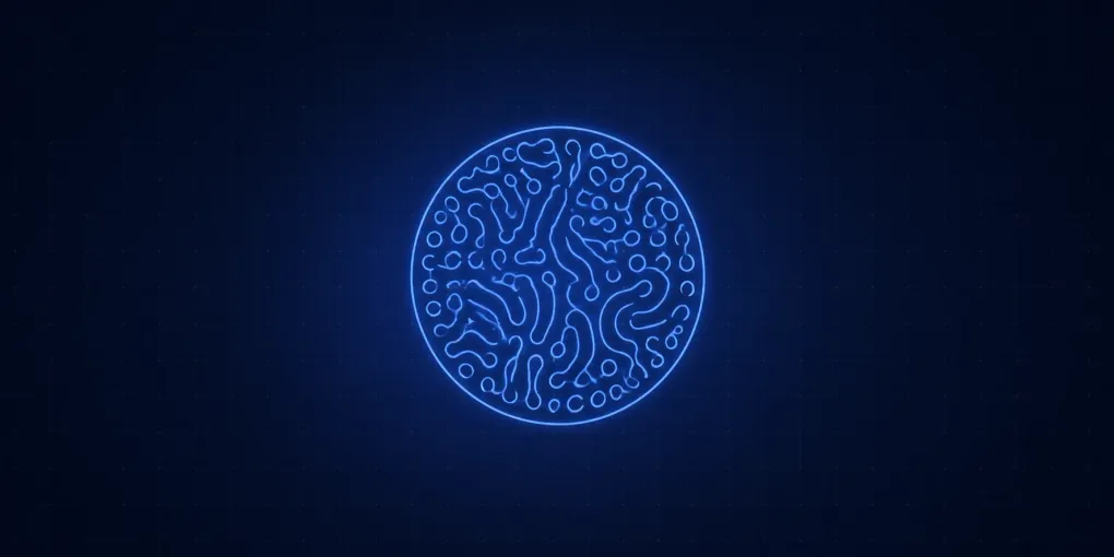
Try the preset menu first. The Stripes preset keeps the reaction active enough for elongated bands to survive. The Spots preset favors separated islands of $B$. The Coral preset creates branching fronts, where local tips can keep advancing while surrounding regions slow down. The Maze preset tends toward connected labyrinth-like forms.

After choosing a preset, move Feed and Kill slowly. Small changes can move the simulation into a different visual regime. That sensitivity is not a bug in the visualization. It is the main point of the model. Reaction-diffusion systems often have parameter regions where a tiny change in rates shifts the attractor: spots may stretch into stripes, stripes may split into branching fronts, or the whole field may wash out.

The Diffusion ratio control changes how fast $B$ diffuses relative to $A$. When the ratio is lower, $B$ remains more localized and sharper features can persist. When the ratio rises, $B$ spreads more easily, so boundaries soften and some fine structure collapses. Pattern formation depends on this mismatch because the two chemicals do not smooth out at the same rate. If everything diffused identically and reactions did not amplify differences, the surface would tend toward bland uniformity.

Time Evolution and Pattern Maturity

Reaction-diffusion patterns are not drawn in one pass. They mature through repeated local updates. Early frames often show expanding rings or rough blobs. Later frames reveal whether those fronts stabilize, fragment, or collide with other structures.

Pause the simulation and use Step to advance it manually. Each step performs the same local rule everywhere on the grid. No step has global knowledge of the future pattern. The emerging structure comes from accumulation: a boundary that was slightly favorable for $B$ becomes more favorable after a few updates, while a starved region loses $B$ and becomes background again.

The Speed slider changes how many simulation updates run per animation frame. At low speed, you can watch fronts move and split. At high speed, the pattern appears to crystallize quickly because many local decisions are being made between rendered frames. This is similar to watching plant growth or colony expansion in time lapse. The final shape looks static, but it is the record of a dynamic process.

For interpretation, it helps to separate transient behavior from long-term behavior. A transient is what happens while the system is still reacting to the initial disturbance. Long-term behavior is what remains after the field has had time to settle into a stable, oscillating, or unstable regime. Two parameter settings can look similar during the first few seconds and then diverge dramatically later. That is why time controls matter: pattern formation is not only about the destination, but also about the path used to get there.

Stable and Chaotic Regions

Not every parameter region produces a clean repeating pattern. Some settings settle into a stable arrangement of spots or stripes. Others produce moving fronts, repeated splitting, or turbulent-looking activity that never fully freezes. The boundary between these regions is one reason reaction-diffusion simulations are so visually compelling.

The left side uses a parameter region that tends to settle into stable spots. The right side uses a more unstable region. Move Chaos pressure to push the right simulation through a range where fronts become more active and less predictable. The same numerical update rule is being used on both sides. The difference is the balance between feed, removal, and diffusion.

This comparison is also a warning against overinterpreting one attractive image. A single still frame might look like coral, lichen, zebra stripes, or cell growth, but the underlying dynamics may be very different. A stable spot pattern and a chaotic front can both produce organic texture. To understand the system, watch how it responds to perturbation, how it changes over time, and whether it returns to a stable arrangement after disturbance.

Why Stripes, Spots, and Branches Appear

The visual categories are easier to understand if you focus on boundaries. Inside a large region of $B$, chemical $A$ may be depleted, so the reaction cannot continue strongly everywhere. Outside the region, $B$ may be too low to reproduce. The boundary is special because both chemicals can coexist there. That is where growth, splitting, and edge sharpening happen.

Spots form when active regions remain localized. The surrounding area supplies enough $A$ for each island to maintain itself, but not enough for every island to expand without limit. Stripes and mazes form when active regions stretch and connect before settling. Branching fronts appear when tips keep finding fresh $A$ while neighboring regions inhibit each other.

This connects to Alan Turing’s original insight about morphogenesis. Turing showed that diffusion, which normally seems like a smoothing process, can help create structure when it is coupled to reactions and different substances diffuse at different rates. The important idea is not that every zebra stripe is literally produced by this exact two-variable Gray-Scott equation. The important idea is that local chemical interaction plus unequal spreading can break symmetry and organize space.

Discrete Simulation Versus Continuous Equations

The equations describe continuous fields, but the browser simulation uses a finite grid. Each cell stores the current $A$ and $B$ concentrations. At every update, the code estimates diffusion by comparing a cell with its neighbors, applies the reaction terms, clamps concentrations to a valid range, and swaps the new field into place.

This approximation is enough for learning because the qualitative behavior is visible. It is not meant to be a laboratory-grade chemical solver. Grid resolution, time step, boundary handling, and numerical stability all affect the final image. For example, too large a time step can make the system unstable for numerical reasons rather than model reasons. Too coarse a grid can make thin bands vanish or lock to pixel directions.

Those limitations are also useful in generative art and graphics. Artists often tune the grid scale, palette, seed, and update rate as part of the aesthetic. The simulation is still driven by mathematical dynamics, but the rendered texture is shaped by implementation choices. That makes reaction-diffusion a good bridge between scientific modeling and procedural graphics. For related procedural texture intuition, the article on noise functions, Perlin noise, and fractal noise is a useful complement: noise injects structured randomness, while reaction-diffusion evolves structure through local dynamics.

Practical Workflow for Exploring a Reaction-Diffusion System

When working with reaction-diffusion models, use a simple exploration loop:

1. Start with a mostly uniform field and a small disturbance.
2. Choose a known stable parameter preset.
3. Change one parameter at a time while watching the pattern over enough time.
4. Paint or perturb the field to test whether the pattern recovers or changes regime.
5. Compare still images with time evolution before deciding what the system is doing.

This workflow avoids a common mistake: treating reaction-diffusion as a static texture generator only. The texture is a trace of a process. If you only tune for a beautiful screenshot, you may miss whether the system is stable, slowly expanding, oscillating, or numerically fragile.

Summary

Reaction-diffusion systems create organic patterns from local rules. In the Gray-Scott model, chemical $A$ is replenished, chemical $B$ is removed, the two react locally, and both diffuse across a surface. From those simple ingredients, the field can produce spots, stripes, maze-like bands, coral-like fronts, and unstable chaotic regions.

The key intuition is that diffusion does not always erase structure. When diffusion is coupled to nonlinear reaction and unequal rates, it can help organize space. That is why reaction-diffusion is such a strong teaching example for emergent behavior: the equations are small, the visuals are immediate, and the connection between math, biology, and generative art is visible directly on the page.