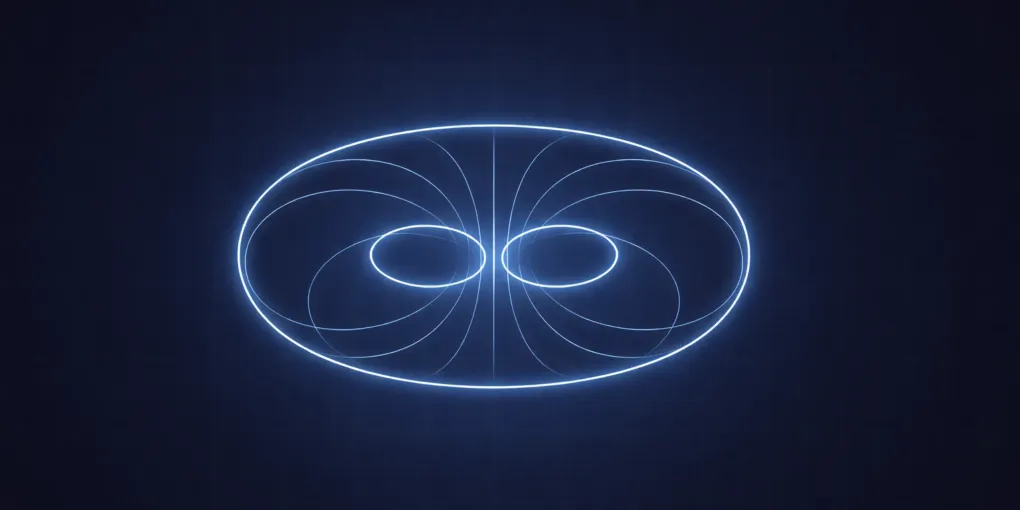
A magnet holds a shopping list to the fridge and swings a compass needle, yet nothing visible passes between the magnet and the thing it moves. The push and pull arrive through empty space, which is what makes magnetism slippery at first. It helps to build the idea in three steps instead of reaching for the full theory at once.

The first step is the field, the invisible arrangement of direction and strength that fills the space around a magnet or a current-carrying wire. The second is force, how that field nudges a moving charge off its path. The third is induction, how a changing field drives current through a nearby loop of wire. Follow those three and electricity and magnetism stop looking like separate subjects. They become two faces of one set of laws, and light falls out of the same laws as part of the bargain.

This page works through the three steps with an interactive model for each: a wire whose current you can raise, a charged particle you can steer through a field, and a flux you can drive back and forth.

Magnetic Fields: Direction and Strength at Every Point

Place a compass beside a bar magnet and its needle locks onto a direction. Move the compass to a new spot and the needle settles on a different one. The needle is reading the local magnetic field, which means that at every point in space there is a direction the field points and a strength attached to it.

Field lines are the standard way to draw that map. Outside a bar magnet they run from the north pole to the south pole; inside the magnet they continue from south back to north, closing into loops. Because the loops never end, a magnet always has both a north and a south pole, no matter how finely you cut it. Line density carries the strength: lines packed close together mark a strong field, and lines spread apart mark a weak one.

These lines are a drawing convention, not physical threads. A compass needle lines up with the tangent to the line at its location, and nothing actually flows along the curve. The picture is a compact way to read direction and relative strength at a glance.

Every magnetic field comes from electric charge in motion. In a permanent magnet, electrons carry tiny magnetic moments, and in iron-like materials many of those moments line up in patches called domains. When enough domains point the same way, the combined field is strong enough to feel from outside the material. A current-carrying wire is the cleaner case to start with, because the motion is a steady drift of charge in one direction.

The Field Around a Current-Carrying Wire

Send a steady current down a long straight wire and the field wraps around the wire in circles. Close to the wire the circles are tight and the field is strong; farther out they spread and weaken. For a wire carrying current $I$, the field magnitude at distance $r$ is

$$B = \frac{\mu_0 I}{2\pi r}$$

$\mu_0$ is the permeability of free space, a constant that sets how strongly a given current produces a magnetic field in a vacuum. Two consequences fall straight out of the formula. Double the current and you double the field. Double the distance and you halve the field, because the strength falls with $1/r$.

The model below shows the wire end-on, as if you were looking down at it from above, with small arrows standing in for compass needles. Near the wire the arrows are long and the rings are tight; moving outward, the field weakens roughly in inverse proportion to distance, so the local arrow shrinks by half each time the distance doubles. Raising the current lengthens every arrow at once and brightens the rings, which is the linear dependence on $I$ made visible. Reversing the current, from a dot to a cross, reverses every arrow and flips the circulation from counterclockwise to clockwise.

The readout is worth watching against a familiar scale. A 10 A current at 10 cm gives about 20 microtesla, the same order of magnitude as Earth’s field at the surface. So the field near an everyday wire is comparable to the planet you live on, and a compass can register it.

How a Magnetic Field Bends a Moving Charge

A magnetic field ignores a charge that is standing still. The moment the charge moves, a force appears that is perpendicular to both the velocity and the field:

$$\mathbf{F} = q,\mathbf{v} \times \mathbf{B}$$

$q$ is the charge, $\mathbf{v}$ is its velocity, and $\mathbf{B}$ is the local magnetic field. The cross product is the important part. It says the force points sideways to the motion rather than along it, so the field cannot speed the particle up or slow it down. It can only steer, which is why a magnetic field bends a moving charge into a curve and leaves its speed unchanged.

Steering a moving charge in a uniform field produces a circle, because the force always turns the velocity by a quarter turn. The radius of that circle is

$$r = \frac{mv}{qB}$$

where $m$ is the particle mass. Faster particles carve wider circles, stronger fields pull them into tighter ones, and heavier particles resist the turn. That relationship powers devices such as the mass spectrometer, which sorts particles by how sharply a field bends them.

Direction is the part that trips people up, so it is worth working on separately from the numbers. For a positive charge, the right-hand rule applied to $\mathbf{v} \times \mathbf{B}$ gives the force direction. For a negative charge such as an electron, compute the same cross product and then reverse the result, because the sign of $q$ flips the force.

The model below shows the same law in motion: a charged particle circling in a uniform field that points out of or into the screen. The blue arrow is velocity and the red arrow is force, and the right angle between them stays fixed as the particle turns. A longer velocity arrow means a faster particle, and the circle widens in direct proportion; a stronger field pulls the same speed into a tighter loop, which is the radius formula $r = mv/(qB)$ behaving on screen. Changing the sign of the charge or the direction of the field reverses the bend while the speed stays constant. Working out the direction with the right hand and the magnitude with the formula covers both halves of the problem.

Ampere’s Law: Coils and Cores Strengthen the Field

The wire formula is one case of a more general statement, Ampere’s law. In plain terms it says that the total magnetic circulation around a closed loop equals the net current threading through that loop, scaled by $\mu_0$:

$$\oint \mathbf{B}\cdot d\mathbf{l} = \mu_0 I_{\text{enc}}$$

The left side adds up the field along a chosen closed path, and $I_{\text{enc}}$ is the current passing through the area that path encloses. For the straight wire, picking a circular path around it reproduces $B = \mu_0 I / 2\pi r$ directly, which is a good check that the two statements agree.

The law explains why a coil beats a straight wire. Wrap the wire into $N$ turns and every turn threads the same path, so the contributions add and the field near the axis grows roughly in proportion to $N$. Coils are how a modest current becomes a field strong enough to move a motor or throw a relay.

It also explains the iron core. A ferromagnetic core responds to the field by aligning its own domains, and that response adds to the flux the current already produced. The same current through the same coil then yields a much stronger field with the core than without it. That is why relays, motors, and transformers put iron or another magnetic material inside their coils instead of leaving them full of air.

There is one more term in the full version of Ampere’s law, added by Maxwell, that matters when the electric field is changing. It comes back in the last section, where it turns out to be the piece that lets light travel.

Faraday’s Law: A Changing Field Drives a Current

Magnetism can also produce electricity, and it needs a change rather than a steady state. Wiggle a magnet near a loop of wire and a current appears in the loop; hold the magnet still and the current stops, even though the field is still there. The trigger is a changing magnetic flux, written $\Phi_B$, which counts the amount of field passing through the loop.

Faraday’s law states that the induced voltage around the loop equals the rate at which flux changes:

$$\mathcal{E} = -\frac{d\Phi_B}{dt}$$

$\mathcal{E}$ is the induced voltage and $d\Phi_B/dt$ is how fast the flux changes. The minus sign is Lenz’s law, and it says the induced current pushes back against the change that created it. Push a magnet toward the loop and the loop generates a current whose field opposes the approach; pull it away and the current flips to resist the retreat. The opposition is nature’s way of making you do work for the energy the current carries.

Written locally rather than around a loop, Faraday’s law says that a magnetic field which varies in time produces a circulating electric field:

$$\nabla \times \mathbf{E} = -\frac{\partial \mathbf{B}}{\partial t}$$

The curl symbol on the left is the local version of circulation around a tiny loop. The key point is that this works in empty space. No wire is required. A changing magnetic field creates an electric field in the surrounding space, and a wire placed there simply gives the induced field a path to drive current along.

The model below pairs a loop of wire with a graph of the flux passing through it. The blue curve is that flux and the red curve is the induced circulation, and a single marker carries both through one full cycle. The blue curve changes fastest where it crosses zero, and there the red curve reaches its largest value. At the blue peaks the rate of change drops to zero and the red curve passes through zero with it. The loop on the left makes the same point: its field markers fill and empty while the induced current around its rim follows the slope of the flux, not its level.

The size of the induced effect depends on how fast the flux moves, so a higher frequency drives the red curve to a larger amplitude even when the blue curve keeps the same height. This is the behavior that runs generators and transformers. A generator keeps the flux through its coils changing so that voltage keeps appearing, and a transformer leans on alternating current precisely because AC keeps the flux in motion.

Maxwell’s Addition and the Origin of Light

Faraday’s law runs one way, from a changing magnetic field to a circulating electric field. Maxwell asked whether the reverse could work and found that it does, provided one extra term is added to Ampere’s law. A changing electric field also produces a circulating magnetic field:

$$\nabla \times \mathbf{B} = \mu_0 \mathbf{J} + \mu_0 \epsilon_0 \frac{\partial \mathbf{E}}{\partial t}$$

$\mathbf{J}$ is the current density, and the new term on the right is Maxwell’s displacement current, proportional to how fast the electric field changes. The first term is the Ampere’s law effect from the wire; the second is the piece that couples a changing electric field back to magnetism.

With both directions of coupling in place, a self-sustaining wave becomes possible. A changing electric field generates a magnetic field, that changing magnetic field generates an electric field, and the pattern marches through space on its own without any charges or wires to carry it. The speed of that wave follows from the two constants:

$$c = \frac{1}{\sqrt{\mu_0 \epsilon_0}}$$

Plug in the measured values of $\mu_0$ and $\epsilon_0$ and $c$ comes out at roughly $3 \times 10^8$ m/s, which was already known as the speed of light. That match is the evidence that light is an electromagnetic wave, and radio, microwaves, infrared, visible light, and X-rays are the same phenomenon at different frequencies. If you want to see that wave nature do physical work, diffraction and the Airy disk shows how the spreading wave sets the resolution limit of any lens.

The remaining two of Maxwell’s equations cover the sources rather than the coupling. Electric charges create electric field, and there are no magnetic charges to create magnetic field, which is the formal statement that field lines never end on a pole.

Common Mistakes and a Practical Workflow

A handful of mistakes show up again and again when people work magnetism problems for the first time. The most common is mixing up the direction of the field with the direction of the force. The field points one way, and the force on a moving charge points sideways to both the field and the motion, so the two rarely align.

The second is forgetting that magnetic force requires motion. A charge at rest in a magnetic field feels nothing from that field, even a strong one, so a problem that seems to be missing a force may simply be missing a velocity.

The third is dropping the sign of the charge. Electrons bend the opposite way from protons in the same field, and ignoring the negative sign flips the answer.

The fourth is confusing flux with the rate of change of flux. Induction depends on how fast the flux changes, so a large steady flux induces nothing while a small flux changing quickly can induce a lot.

When a problem looks unfamiliar, a short routine keeps it grounded. Sketch the velocity, field, and geometry before touching any formula. Decide which law fits, whether it is the wire field, the force law, Ampere’s law, or Faraday’s law. Predict the direction first, then compute the magnitude. Sanity-check that magnitude against everyday scales such as microtesla for Earth’s field and millitesla to tesla for strong magnets. Finally, test a limiting case such as zero velocity or constant flux and see whether the result still makes sense.

Recap

Magnetism is the visible side of electric charge in motion. Charges that drift or align produce a magnetic field, and that field steers other moving charges sideways without changing their speed. Ampere’s law ties the field to the current that creates it, and adding an iron core or more turns concentrates the effect into the strong fields that run motors and transformers.

Changing the picture in time adds the second half of the story. Faraday’s law turns a changing magnetic flux into a circulating electric field and an induced voltage, while Maxwell’s extra term lets a changing electric field create magnetic field in return. That mutual coupling carries a wave through empty space at the speed of light, which places electricity, magnetism, and light inside a single framework. Once you can move between the field picture, the direction rules, and the equations, the behavior becomes something you can predict.